3. Synthetic Populations and HDF5 I/O
If you are going to simulate the accretion of thousands of planets, using a numpy array is computationally vital. Additionally, PA3Py provides native methods to save the entire population to disk (.h5).
[1]:
import sys
import os
import numpy as np
sys.path.insert(0, os.path.abspath('../../src'))
from pa3py import PA3Py

# Initialize the engine
sim = PA3Py('../../tests/test_data/run_smooth_a0.001_v10')
[load_tripodpy_hdf5] Reading 100 snapshots from ../../tests/test_data/run_smooth_a0.001_v10...
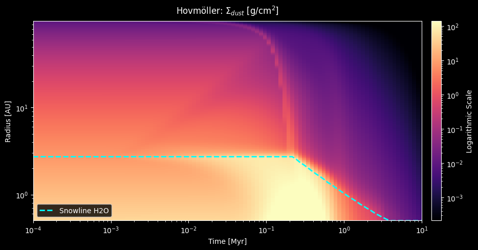
Plotting the Hovmöller Diagram
Before placing embryos, it is useful to visualize the snowlines over the disk.
Hovmöller Diagram Fields The plot_hovmoller() function supports three different fields for visualization. You can change them using the field argument:
field='dust_Sigma'(default): Displays the surface density of dust (\(\Sigma_{\rm dust}\)) in g/cm\(^2\).field='gas_Sigma': Displays the surface density of gas (\(\Sigma_{\rm gas}\)) in g/cm\(^2\).field='epsilon': Displays the dust-to-gas mass ratio (\(\epsilon = \Sigma_{\rm dust} / \Sigma_{\rm gas}\)).
[2]:
import matplotlib.pyplot as plt
sim.plot_hovmoller(field='dust_Sigma', show_snowlines=True)
plt.show()
Defining the Synthetic Population
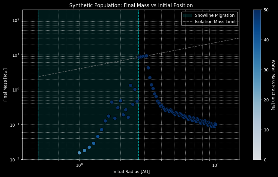
We will use np.linspace to generate 100 embryos along the disk.
[3]:
# Important: to avoid infinite decimals (e.g. 1.98989), we use 99 points
# for a range of 98 units (1 to 99) to ensure integer steps.
embryos = np.linspace(1.0, 10.0, 99).tolist()

# If you don't need to print the keys, using np.linspace(1, 99, 100) is perfectly valid.

print("Simulating", len(embryos), "embryos...")
results = sim.run_growth(embryos)
Simulating 99 embryos...

-------------------------------------------------------------
  r [AU]  M_tot [ME]  M_iso [ME]  f_silicates[%]  f_H2O[%]
-------------------------------------------------------------
    1.00        0.015         3.96            71.3      28.7
    1.09        0.018         4.22            67.6      32.4
    1.18        0.022         4.49            64.7      35.3
    1.28        0.029         4.75            61.2      38.8
    1.37        0.045         5.00            57.3      42.7
    1.46        0.071         5.25            54.1      45.9
    1.55        0.126         5.50            51.9      48.1
    1.64        0.174         5.74            51.2      48.8
    1.73        0.438         5.98            50.4      49.6
    1.83        0.151         6.21            51.3      48.7
    1.92        0.303         6.45            50.5      49.5
    2.01        0.477         6.68            52.3      47.7
    2.10        0.189         6.91            50.8      49.2
    2.19        0.264         7.13            50.5      49.5
    2.29        0.161         7.35            51.1      48.9
    2.38        1.323         7.57            50.1      49.9
    2.47        0.377         7.79            50.3      49.7
    2.56        1.013         8.01            50.1      49.9
    2.65        0.467         8.22            50.3      49.7
    2.74        8.434         8.43            50.0      50.0
    2.84        8.646         8.65            50.0      50.0
    2.93        8.855         8.86            50.0      50.0
    3.02        9.063         9.06            50.0      50.0
    3.11        9.267         9.27            50.0      50.0
    3.20        4.200         9.47            50.0      50.0
    3.30        2.199         9.68            50.0      50.0
    3.39        1.367         9.88            50.0      50.0
    3.48        1.067        10.08            50.0      50.0
    3.57        0.749        10.28            50.1      49.9
    3.66        0.632        10.47            50.1      49.9
    3.76        0.466        10.67            50.1      49.9
    3.85        0.411        10.86            50.1      49.9
    3.94        0.337        11.06            50.1      49.9
    4.03        0.344        11.25            50.1      49.9
    4.12        0.305        11.44            50.2      49.8
    4.21        0.276        11.63            50.2      49.8
    4.31        0.252        11.82            50.2      49.8
    4.40        0.275        12.01            50.2      49.8
    4.49        0.254        12.20            50.2      49.8
    4.58        0.235        12.39            50.2      49.8
    4.67        0.261        12.57            50.2      49.8
    4.77        0.243        12.76            50.2      49.8
    4.86        0.226        12.94            50.2      49.8
    4.95        0.210        13.12            50.2      49.8
    5.04        0.196        13.31            50.3      49.7
    5.13        0.221        13.49            50.2      49.8
    5.22        0.206        13.67            50.2      49.8
    5.32        0.193        13.85            50.3      49.7
    5.41        0.180        14.03            50.3      49.7
    5.50        0.206        14.21            50.2      49.8
    5.59        0.192        14.38            50.3      49.7
    5.68        0.180        14.56            50.3      49.7
    5.78        0.168        14.73            50.3      49.7
    5.87        0.158        14.91            50.3      49.7
    5.96        0.183        15.09            50.3      49.7
    6.05        0.171        15.26            50.3      49.7
    6.14        0.160        15.43            50.3      49.7
    6.23        0.150        15.61            50.3      49.7
    6.33        0.141        15.78            50.4      49.6
    6.42        0.166        15.95            50.3      49.7
    6.51        0.156        16.12            50.3      49.7
    6.60        0.146        16.29            50.3      49.7
    6.69        0.137        16.46            50.4      49.6
    6.79        0.129        16.63            50.4      49.6
    6.88        0.154        16.80            50.3      49.7
    6.97        0.144        16.97            50.3      49.7
    7.06        0.136        17.13            50.4      49.6
    7.15        0.128        17.30            50.4      49.6
    7.24        0.120        17.47            50.4      49.6
    7.34        0.145        17.63            50.3      49.7
    7.43        0.136        17.80            50.4      49.6
    7.52        0.128        17.96            50.4      49.6
    7.61        0.121        18.13            50.4      49.6
    7.70        0.116        18.29            50.4      49.6
    7.80        0.110        18.45            50.5      49.5
    7.89        0.130        18.62            50.4      49.6
    7.98        0.124        18.78            50.4      49.6
    8.07        0.117        18.94            50.4      49.6
    8.16        0.111        19.10            50.5      49.5
    8.26        0.105        19.26            50.5      49.5
    8.35        0.126        19.42            50.4      49.6
    8.44        0.119        19.59            50.4      49.6
    8.53        0.113        19.74            50.4      49.6
    8.62        0.107        19.90            50.5      49.5
    8.71        0.102        20.06            50.5      49.5
    8.81        0.096        20.22            50.5      49.5
    8.90        0.116        20.38            50.4      49.6
    8.99        0.110        20.53            50.5      49.5
    9.08        0.104        20.69            50.5      49.5
    9.17        0.098        20.85            50.5      49.5
    9.27        0.093        21.01            50.5      49.5
    9.36        0.089        21.16            50.6      49.4
    9.45        0.106        21.32            50.5      49.5
    9.54        0.101        21.47            50.5      49.5
    9.63        0.095        21.62            50.5      49.5
    9.72        0.091        21.78            50.6      49.4
    9.82        0.088        21.93            50.6      49.4
    9.91        0.104        22.09            50.5      49.5
   10.00        0.099        22.24            50.5      49.5
-------------------------------------------------------------
[4]:
# Generar el gráfico completo de la población usando el método nativo
fig, ax = sim.plot_population(results)
plt.xlim(0,15)
plt.show()
C:\Users\Maxlo\AppData\Local\Temp\ipykernel_40752\670884697.py:3: UserWarning: Attempt to set non-positive xlim on a log-scaled axis will be ignored.
  plt.xlim(0,15)
Saving Results (HDF5)
We will save the entire run to the hard drive.
[5]:
sim.save_results(results, "synthetic_population_100.h5")
print("Data saved!")
Data saved!
Loading Results
Tomorrow, when you open this notebook again, you won’t have to re-run the physics.
[6]:
# Load the matrix and also the list of chemistry used in that run
loaded_results, chemistry = PA3Py.load_results("synthetic_population_100.h5")

print("Species from the original simulation:", chemistry)
print("Loaded planets:", len(loaded_results))
Species from the original simulation: ['silicates', 'H2O']
Loaded planets: 99