1. Getting Started with PA3Py
In this notebook, we will learn how to initialize PA3Py, run a growth simulation for an embryo, and plot the results.
[7]:
import sys
import os
import matplotlib.pyplot as plt

# Add package path (if running from the local repository)
sys.path.insert(0, os.path.abspath('../../src'))
from pa3py import PA3Py
from pa3py import constants as c
Initializing the Simulation
We load the simulation simply by passing the path of our HDF5 disk output to the main PA3Py class.
[8]:
# Path to your TripodPy HDF5 data
data_path = '../../tests/test_data/run_smooth_a0.001_v10'

# Initialize the engine
sim = PA3Py(data_path)
[load_tripodpy_hdf5] Reading 100 snapshots from ../../tests/test_data/run_smooth_a0.001_v10...
Running Growth
We will tell PA3Py to compute the growth for an embryo located at 3 AU, with an initial seed mass of \(10^{-3} M_\oplus\).
[9]:
# Embryos to simulate
embryos = [3.0]
# Execute the module
results = sim.run_growth(embryos, m_seed_me=1e-3)
-------------------------------------------------------------
  r [AU]  M_tot [ME]  M_iso [ME]  f_silicates[%]  f_H2O[%]
-------------------------------------------------------------
    3.00        9.016         9.02            50.0      50.0
-------------------------------------------------------------
Plotting Mass Evolution
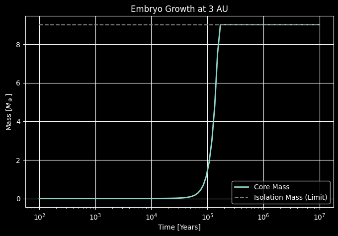
The results dictionary contains arrays where the first column is time (in seconds) and the second is the total mass of the embryo.
[10]:
# Extract data for the embryo at 3 AU
history_3au = results[3.0]

time_years = history_3au[:, 0] / (3.154e7)  # Convert s to years
total_mass = history_3au[:, 1] / c.M_EARTH # Convert to Earth Masses
iso_mass = history_3au[:, 2] / c.M_EARTH


plt.figure(figsize=(8,5))
plt.plot(time_years, total_mass, lw=2, label="Core Mass")
plt.plot(time_years, iso_mass, '--', color='gray', label="Isolation Mass (Limit)")
plt.xlabel("Time [Years]")
plt.ylabel(r"Mass [$M_\oplus$]")
plt.xscale("log")
plt.title("Embryo Growth at 3 AU")
plt.legend()
plt.grid(True)
plt.show()
Water Mass Fraction
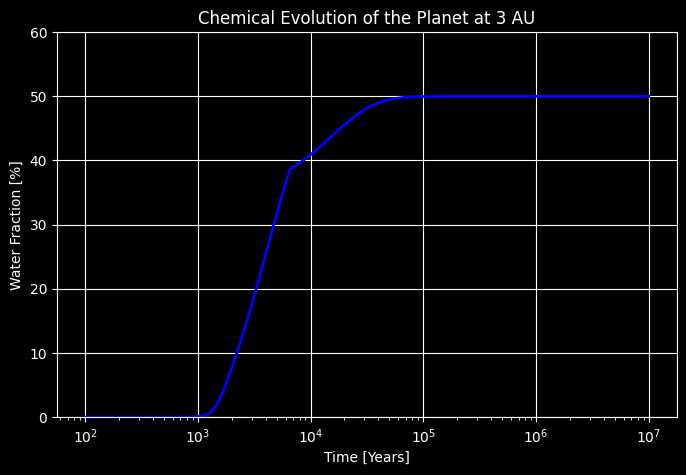
By default, PA3Py runs the classic silicates and H2O model by tracking the dynamic snowline position. We can extract the water mass (column 4) and see how the fraction increased.
[11]:
silicate_mass = history_3au[:, 3]
water_mass = history_3au[:, 4]
total_mass_sum = silicate_mass + water_mass

water_fraction = 100 * water_mass / total_mass_sum

plt.figure(figsize=(8,5))
plt.plot(time_years, water_fraction, color='blue', lw=2)
plt.xscale("log")
plt.xlabel("Time [Years]")
plt.ylabel("Water Fraction [%]")
plt.title("Chemical Evolution of the Planet at 3 AU")
plt.ylim(0, 60)
plt.grid(True)
plt.show()